




What a spatial join does
A spatial join links two layers by location. Each feature of the target layer looks for features of the join layer that have the right spatial relationship to it: it sits inside one, touches one, crosses one, lies within a set distance of one, or is closest to one. When it finds a match, it copies the attributes of the join feature onto the target feature. A normal table join needs a shared ID column. A spatial join needs only that both layers describe the same place.
The geometry of the target layer never changes. If you join store points to sales districts, you get the same store points back, now with a district name, a manager and a region. If you join districts to stores, you get the same districts back, now with a store count and the total sales. When one target feature has several matches, you choose what happens: keep one row per target and combine the values with a merge rule (sum, mean, first, join and more), or write one row per match.
I built this tool to follow the Spatial Join tool in ArcGIS Pro step by step, so anyone who knows ArcGIS finds every parameter where they expect it: target features, join features, join operation, keep all target features, match option, search radius and field map. Drop a zipped Shapefile, GeoJSON, KML, KMZ, GPX or WKT file on the map, pick the layers and click Run Spatial Join. All the work runs in your browser, so your files stay on your computer. The map starts without a basemap, and you can turn one on at any time.
Spatial join, table join, nearest join, identity and intersect: which one do you need?
Many tools combine two layers, and the names are easy to mix up. The difference is what links the two layers and what happens to the geometry. Here they are side by side.
| Tool | What links the layers | Geometry in the output | Attributes in the output |
|---|---|---|---|
| Spatial Join (this tool) | Location, by a match option | Target geometry, unchanged | Target fields plus the join fields you choose, merged by rules |
| Table Join (attribute join) | A shared ID value in a column | Target geometry, unchanged | Target fields plus the table fields |
| Nearest Join (Closest option here) | The shortest distance | Target geometry, unchanged | Target fields plus the nearest feature fields and the distance |
| Identity | Overlap of area | Target cut where it overlaps the second layer | Target fields on every piece, second layer fields on the overlap pieces |
| Intersect | Overlap of area | Only the overlapping parts | Fields of both layers |
| Clip | Overlap of area | Target cut to the clip area | Target fields only |
| Points in Polygon | A point is inside or outside | Points, unchanged | Points split into inside and outside groups |
A quick way to choose: if you want to keep your features whole and read a value from the layer at the same place, use a spatial join. If you need the features cut into pieces so each piece knows its zone, use Identity. If you have a shared ID column and the places do not matter, use a table join.
The match options: how features are matched by location
The match option is the rule that decides which join features belong to a target feature. ArcGIS Pro lists 16 options. This table lists 14, because ArcGIS has a flat (planar) and a geodesic version of Within a distance and of Closest, and this tool always measures on the Earth, which is the geodesic version. The spatial relationships follow the DE-9IM model, the same model that PostGIS, GEOS, JTS and QGIS use.
| Match option | ArcGIS Pro keyword | A join feature matches when | Typical use |
|---|---|---|---|
| Intersect | INTERSECT | The two features share at least one point. They overlap, cross, touch, or one holds the other. | Tag each point with the county polygon it falls in. |
| Within a distance | WITHIN_A_DISTANCE_GEODESIC | The shortest distance between the two features is not larger than the search radius, measured on the Earth in metres. | Find every clinic within 500 m of a bus stop. |
| Contains | CONTAINS | The target feature contains the join feature. The join feature may touch the target border. | Count the trees inside each park. |
| Completely contains | COMPLETELY_CONTAINS | The join feature is inside the target feature and does not touch its border at all. | Find parcels that hold a well well away from the fence line. |
| Contains (Clementini) | CONTAINS_CLEMENTINI | Like Contains, but a join feature that lies only on the target border does not match. The insides must meet. | Count points in a polygon and skip points exactly on its edge. |
| Within | WITHIN | The target feature is inside the join feature. The target may touch the join border. | Tag each building with its zoning polygon. |
| Completely within | COMPLETELY_WITHIN | The target feature is inside the join feature and does not touch its border at all. | Keep only the buildings that are fully inside a flood zone. |
| Within (Clementini) | WITHIN_CLEMENTINI | Like Within, but a target that lies only on the join border does not match. The insides must meet. | Tag points with a district and ignore points on the district border. |
| Are identical to | ARE_IDENTICAL_TO | The two features have exactly the same geometry. | Link two versions of the same boundary layer. |
| Boundary touches | BOUNDARY_TOUCHES | The borders touch, but the insides do not overlap. | List the neighbours of each parcel. |
| Share a line segment with | SHARE_A_LINE_SEGMENT_WITH | The two features share a stretch of line, which is more than a single point. | Find the roads that run along a county border. |
| Are crossed by the outline of | CROSSED_BY_THE_OUTLINE_OF | The outline of the join feature crosses the target feature at a point, and the two features do not merely touch. | Find the rivers that cross each municipality. |
| Have their center in | HAVE_THEIR_CENTER_IN | The center of the target feature is inside the join feature. A point is its own center, a line uses its midpoint, a polygon uses its centroid. | Give each large polygon to the one region that holds its center. |
| Closest | CLOSEST_GEODESIC | The one join feature with the shortest distance to the target feature. The search radius is optional. | Find the nearest hospital for each address. |
If you are not sure, start with Intersect. It works for point in polygon, line in polygon and polygon in polygon. Switch to Within or Contains when you want to be strict about which feature holds which, and to a Clementini option when points on a border must not match.
Join operation, keep all target features and the other parameters
These parameters are the same ones you see in the ArcGIS Pro tool pane. They decide how many output rows you get and which fields they carry.
- One to one. Each target feature gives exactly one output row. If several join features match, the merge rules of the field map combine their values into one. Use it to tag each point with its polygon, or to total the sales inside each district.
- One to many. Each match gives its own output row, so one target feature can appear several times, each time with the attributes of one join feature. Merge rules do not apply. Use it when you need to see every match, for example every flood zone a parcel touches.
- Keep all target features. On (the default in ArcGIS): target features without a match stay in the output, with empty join fields and a Join_Count of 0. Off: only target features with at least one match stay. ArcGIS calls the two settings KEEP_ALL and KEEP_COMMON.
- Search radius. Needed for Within a distance, optional for Closest. Type a number and pick meters, kilometers, feet, yards, miles or nautical miles. For Closest, a radius leaves a feature unmatched when nothing lies inside it.
- Distance field. For Within a distance and Closest, tick the box to add the distance of the match, in metres, as the field
Join_Distance_m. In one to one, it is the shortest distance among the matches. - Join_Count and TARGET_FID. The tool always adds these two fields, as ArcGIS does. Join_Count is the number of join features that matched the target. TARGET_FID is the position of the target feature in its layer, starting at 0, so you can trace every output row back to its source.
- Field map. The field map lists the fields of the join layer. For each one you choose whether to add it, how several matches are merged (one to one only) and the output name. The next section explains the merge rules.
Merge rules: what happens when one feature has several matches
In a one to one join, a target feature with several matches still gets one row. The merge rule of each field decides which value goes into that row. This is the same idea as the merge rules in the ArcGIS Pro field map.
| Merge rule | Works on | The value in the output |
|---|---|---|
| First | Any field | The value of the first match, in the order of the join layer. |
| Last | Any field | The value of the last match, in the order of the join layer. |
| Join (text) | Any field | All values written into one text, in layer order, with the delimiter between them (a comma and a space by default). |
| Sum | Number fields | The total of all values. |
| Mean | Number fields | The average of all values. |
| Median | Number fields | The middle value. With an even count, the mean of the two middle values. |
| Mode | Any field | The value that appears most often. When two values tie, the one found first wins. |
| Minimum | Number fields | The smallest value. |
| Maximum | Number fields | The largest value. |
| Standard deviation | Number fields | The population standard deviation of the values (the sum of squares is divided by n). |
| Count | Any field | How many matches have a value in this field. The result is a whole number. |
Empty values are ignored by every rule. If no match has a value, the output is empty (0 for Count). Text fields can use First, Last, Join, Count and Mode. A field counts as a number field when all its values are numbers, so a column of numbers stored as text needs to be converted first.
Other names for the spatial join
The same operation has different names in different software, and people search for all of them. Here is where each name points.
| Name you may know | Where you see it | What it means |
|---|---|---|
| Spatial Join | ArcGIS Pro, ArcMap, arcpy | The original name. Analysis toolbox > Overlay > Spatial Join, and arcpy.analysis.SpatialJoin. |
| Add Spatial Join | ArcGIS Pro | The same matching, but it joins on the fly to a layer and writes no new data. |
| Join Features | ArcGIS Online, Map Viewer | The web version of the analysis. You pick a spatial relationship and a join operation. |
| Join attributes by location | QGIS | Under Vector > Data Management Tools. It has the summary version (join statistics) and a separate Join attributes by nearest tool. |
| sjoin and sjoin_nearest | GeoPandas | geopandas.sjoin(left, right, how, predicate) and geopandas.sjoin_nearest for the closest match. |
| st_join | R (sf package) | st_join(x, y, join = st_within, left = TRUE) gives a left join by location. |
| ST_Intersects, ST_Within or ST_DWithin in a JOIN | PostGIS, BigQuery, SQL Server, Snowflake | A normal SQL join with a spatial function in the ON clause. |
| Join by location, location join, geo join | Everyday GIS talk | Plain names for the same job. |
| Point in polygon join, tag points with a polygon name | Everyday GIS talk | A spatial join with points as the target and polygons as the join layer. |
| Count points in polygon, summarize within | ArcGIS, QGIS | A spatial join with polygons as the target, points as the join layer, one to one, Join_Count and a Sum rule. |
| Nearest join, join to the closest feature | ArcGIS, QGIS, PostGIS | A spatial join with the Closest match option. |
If you were looking for "how do I add the polygon name to every point in my file", this is the tool.
Supported file formats
You can load several files at once, and you can mix formats. Each file becomes its own layer in the Layers panel. A layer can hold points, lines and polygons together, and each of them is handled with the right method.
Input formats (what you can upload)
| Format | Extension | Notes |
|---|---|---|
| GeoJSON | .geojson, .json | A FeatureCollection, a single Feature or a bare geometry. A GeometryCollection is split into its parts. |
| Esri Shapefile | .zip | Zip the .shp, .shx and .dbf files together. Add the .prj file and projected data is converted to WGS84 when it loads. A .cpg file sets the text encoding. |
| KML | .kml | Google Earth placemarks. MultiGeometry is split into its parts, and ExtendedData becomes attributes. |
| KMZ | .kmz | A zipped KML file. The first .kml file inside the archive is read. |
| GPX | .gpx | GPS files. Waypoints become points, and tracks and routes become lines. Elevation values are kept. |
| WKT | .wkt, .txt | Well-Known Text. One geometry for the whole file, or one geometry per line. |
Output formats (what you can download)
| Format | Extension | Notes |
|---|---|---|
| GeoJSON | .geojson | The standard web format (RFC 7946) in WGS84. Keeps every attribute and its type. Opens in ArcGIS Pro, QGIS and almost every web map library. |
| KML | .kml | Opens in Google Earth. Attributes are written as ExtendedData on each placemark. |
| CSV (WKT) | .csv | One row per feature. The first column holds the geometry as WKT, and each attribute gets its own column. Opens in Excel, and QGIS can read the WKT column as geometry. |
Each file can be up to 50 MB. For very large national datasets, a desktop GIS is still the better choice. See the comparison further down this page.
Technical details
Here is exactly what the tool does with your data. If you know the Spatial Join tool in ArcGIS Pro, most of this will look familiar.
- Layer types
- The target layer and the join layer can each hold points, lines and polygons, including the Multi versions, and one layer can mix them. You can also pick the same layer as target and join layer.
- Target geometry
- Never changed. Every output feature carries the exact geometry of its target feature.
- Output fields
Join_CountandTARGET_FIDfirst, thenJoin_Distance_mif you ticked it, then every field of the target layer, then the join fields you chose.- Field name clashes
- If a join field has the same name as a target field, the target field keeps its name and the join field gets a suffix:
namebecomesname_1, thenname_2, and so on. The results box lists every renamed field. - TARGET_FID
- The position of the target feature in its layer, starting at 0. In one to many it repeats on every row of the same target feature.
- Spatial relationships
- Intersect, Contains, Within, Identical, Boundary touches, Share a line segment with and Are crossed by the outline of use the DE-9IM matrix from the JSTS library. Points against polygons use an indexed point-in-polygon test with the same results.
- Distance
- Within a distance and Closest measure the shortest distance between the two shapes on a sphere with a radius of 6,371,008.8 m, in metres. The distance is 0 when the shapes touch, cross or one holds the other.
- Closest ties
- If two join features are equally close, the one that comes first in the join layer is used. A feature matched against itself (same layer as target and join) has distance 0.
- Order of matches
- First, Last, Join and Mode follow the order of the features in the join layer.
- Boundary rule
- The edge counts as inside for Intersect, Contains and Within. The Completely and Clementini options leave out features that only lie on an edge. See the match options table above.
- Coordinate system
- WGS84 longitude and latitude (EPSG:4326), the same as GeoJSON. A zipped Shapefile with a .prj file is converted to WGS84 when it loads. A feature that crosses the 180th meridian is not wrapped, so split it first.
- Invalid geometry
- An invalid polygon, such as a bow tie, is repaired with a zero-width buffer for the matching only. The output keeps the original geometry. The results box counts the repaired polygons. A geometry that cannot be read never matches.
- Speed
- A grid index limits the join features tested for each target feature. On a normal laptop, 100,000 points against 1,000 detailed polygons takes about one second.
- Privacy
- Everything runs in your browser. No file and no geometry is sent to a server.
How to use the spatial join tool, step by step
Here is the whole workflow with the built-in sample data: a layer of stores with a sales figure, and a layer of four sales districts with a name, a region, a manager and a number of households. The Downtown district overlaps the other three, and some stores lie outside all of them. Your own files work the same way.
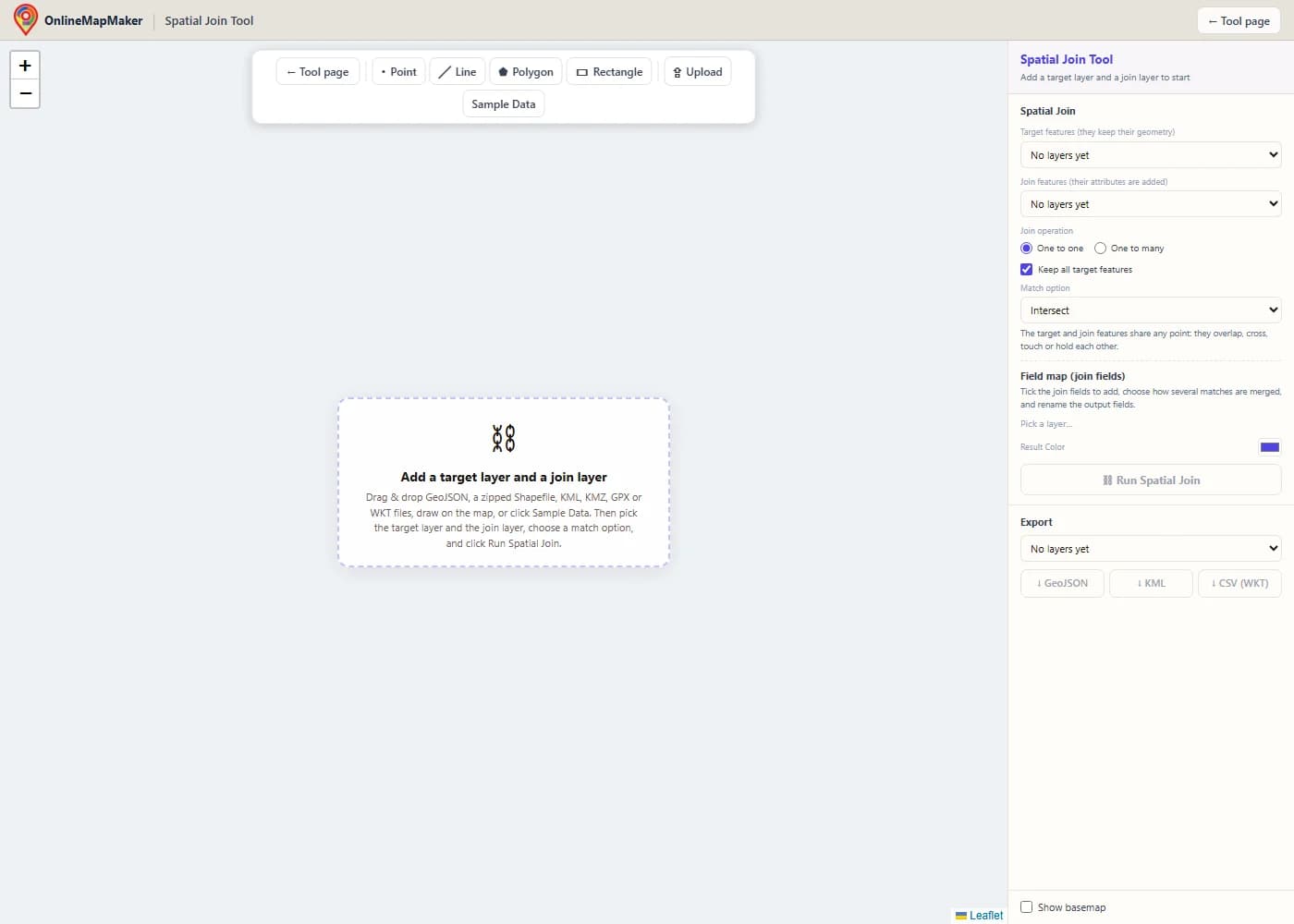
The map opens empty and without a basemap, so nothing loads that you do not need. The toolbar has Point, Line, Polygon and Rectangle drawing tools, an Upload button and a Sample Data button.
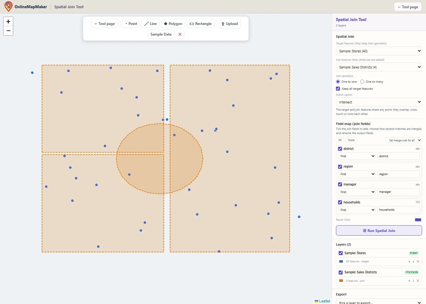
Drag and drop your files onto the map, or click Upload. Here I clicked Sample Data. It adds the stores (blue points) and the sales districts (amber polygons). The first layer you add becomes the target layer, and the second becomes the join layer.
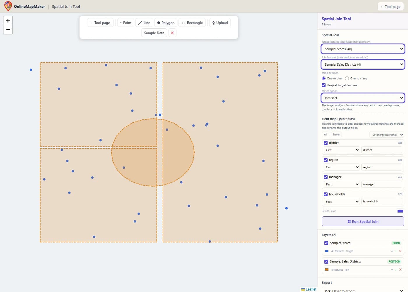
In the Spatial Join panel, choose the target features (they keep their geometry) and the join features (they give their attributes). Then pick One to one or One to many, decide whether to keep all target features, and choose a match option. Under the option you see a short explanation of its rule.
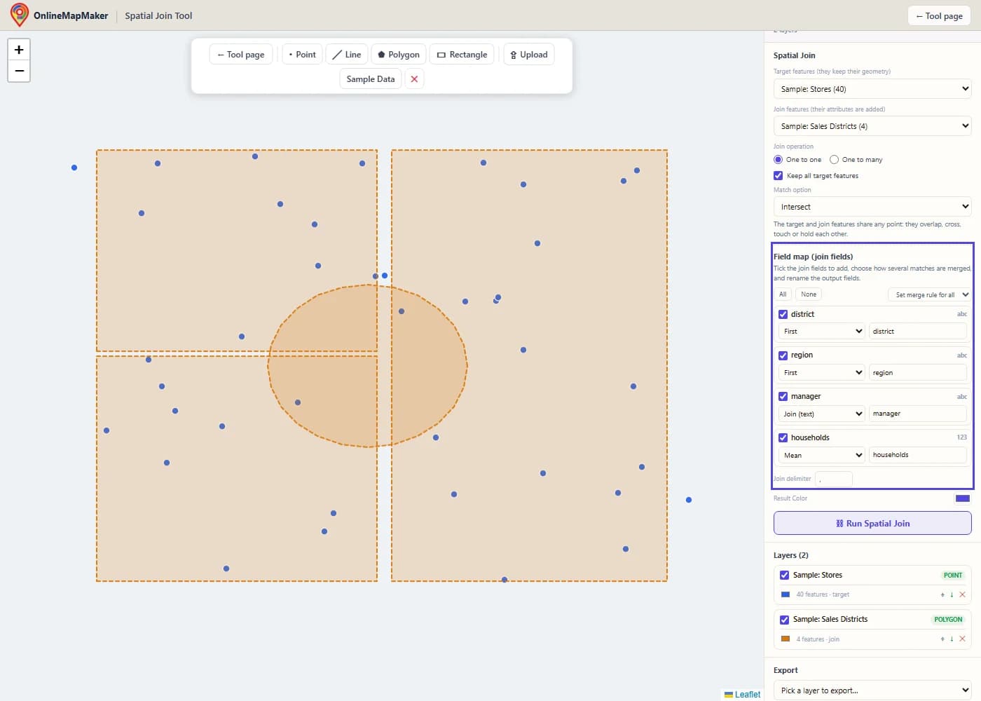
The field map lists every field of the join layer. Tick the ones you want, choose a merge rule for each (First, Join, Sum, Mean and so on) and rename the output fields if you like. The rules are used when a target feature has more than one match.
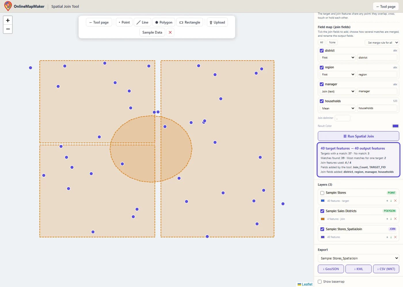
The result appears as a new layer, and the target layer is hidden. The results box shows how many target features found a match and how many did not, the number of matches found, the largest number of matches for one target, and the fields that were added.
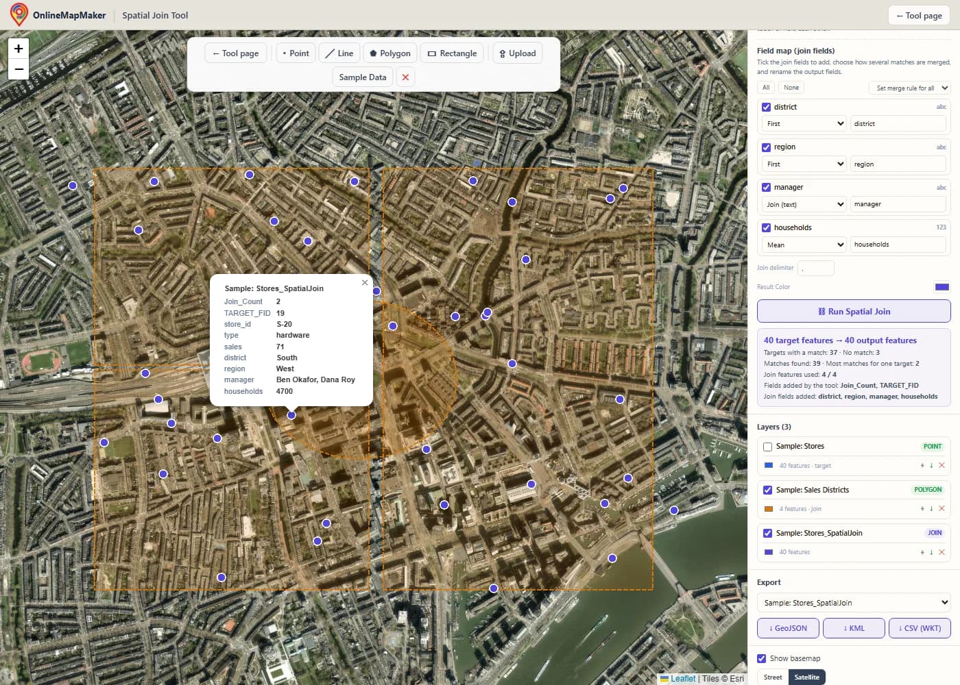
Tick "Show basemap" to see the result on a street or satellite map. Click a store to open its attributes. You see Join_Count and TARGET_FID, then the store fields, then the district fields in one table. A store outside every district shows empty district fields.
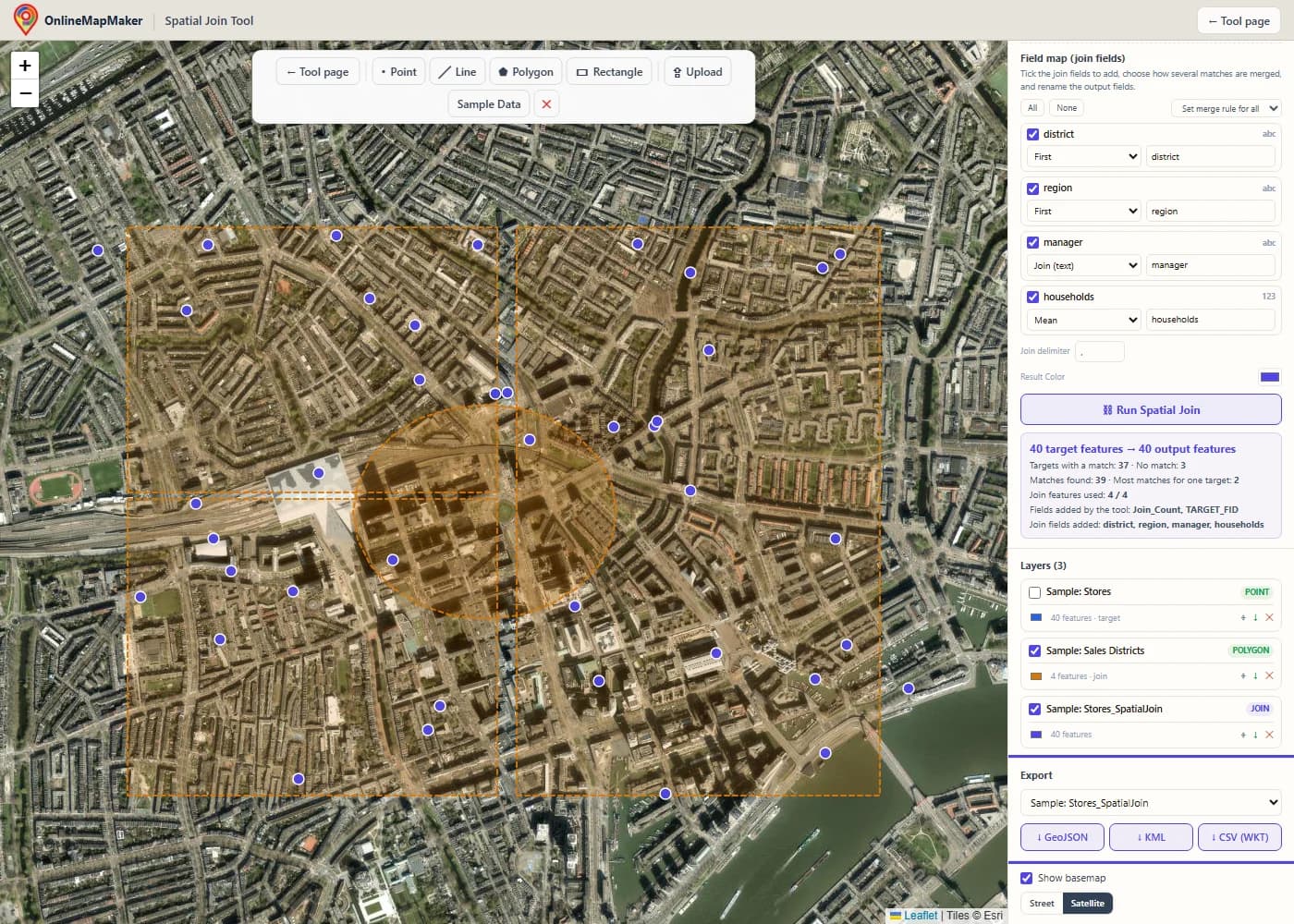
In the Export panel, pick the layer and download it as GeoJSON, KML or CSV with a WKT column. The small arrow next to each layer in the Layers panel is a quick GeoJSON download. To count stores per district, swap the two layers, pick Contains, and set the Sum rule on the sales field.
How to run a spatial join in a GIS
Every GIS has this tool under a different name. ArcGIS calls it Spatial Join, QGIS calls it Join attributes by location, and GeoPandas calls it sjoin. Here is how to do it in this tool, in ArcGIS Pro, in ArcMap, in QGIS and in ArcGIS Online, and how to script it.
In this tool
Load the layer you want to keep and the layer that holds the attributes. Choose the first as the target layer and the second as the join layer. Pick the join operation, the match option and the fields to add, then click Run Spatial Join. Points, lines and polygons in the same layer are all handled in one run. To use a rectangle as the join layer, click Rectangle and click two opposite corners on the map.
In ArcGIS Pro
Open the Geoprocessing pane and search for Spatial Join. It is in the Analysis toolbox under Overlay. Set Target Features and Join Features, choose the output, pick the Join Operation, tick or clear Keep All Target Features, choose a Match Option and set a Search Radius if the option needs one. Use the Field Map to choose fields and merge rules, then click Run. The output has Join_Count and TARGET_FID. To join without writing new data, use Add Spatial Join.
In ArcMap
In ArcMap the tool is in ArcToolbox > Analysis Tools > Overlay > Spatial Join, and the Joins and Relates submenu of a layer also has Join Data > Join data from another layer based on spatial location. The parameters are the same as in ArcGIS Pro, with fewer match options. Esri retired ArcMap in March 2026, so for new work I recommend ArcGIS Pro, QGIS or this tool.
In QGIS
Open Vector > Data Management Tools > Join Attributes by Location. Pick the input layer and the join layer, tick one or more geometric predicates (intersects, contains, equals, touches, overlaps, within, crosses), choose the fields to add, and pick the join type: one feature per match (one to many), the first match only (one to one), or the match with the largest overlap. For statistics such as sum and mean, use Join Attributes by Location (Summary). For the nearest feature, use Join Attributes by Nearest.
In ArcGIS Online (Map Viewer)
Open the layer, choose Analysis, and run Join Features. Pick the target layer, the join layer, a spatial relationship and a join operation, and add statistics for one to one joins. The match options are fewer than in ArcGIS Pro, and the credits are used for hosted analysis, so for a quick one-off job this tool is faster.
With code (arcpy, PyQGIS, GeoPandas, R and SQL)
In ArcGIS Pro the function is arcpy.analysis.SpatialJoin(target_features, join_features, out_feature_class, join_operation, join_type, field_mapping, match_option, search_radius, distance_field_name). The code below shows it, with a Sum merge rule, plus the same job in PyQGIS, GeoPandas, R and PostGIS.
The same spatial join in code
If you run the same join every week, a script saves time. These examples tag stores with the district they are in, find the nearest hospital for each address, and total the sales per district.
import arcpy

arcpy.env.workspace = r"C:\data\city.gdb"

# ArcGIS Pro: Analysis toolbox > Overlay > Spatial Join
arcpy.analysis.SpatialJoin(
    target_features="stores",
    join_features="districts",
    out_feature_class="stores_districts",
    join_operation="JOIN_ONE_TO_ONE",   # or JOIN_ONE_TO_MANY
    join_type="KEEP_ALL",               # or KEEP_COMMON
    match_option="INTERSECT",           # CONTAINS, WITHIN, CLOSEST_GEODESIC ...
)

# Closest, with the distance in a field
arcpy.analysis.SpatialJoin("addresses", "hospitals", "addr_nearest",
    "JOIN_ONE_TO_ONE", "KEEP_ALL",
    match_option="CLOSEST_GEODESIC", search_radius="20 Kilometers",
    distance_field_name="dist_m")

# Total sales per district: a field map with a Sum merge rule
fms = arcpy.FieldMappings()
fms.addTable("districts")                 # keep the target fields
fm = arcpy.FieldMap()
fm.addInputField("stores", "sales")
fm.mergeRule = "Sum"
out = fm.outputField
out.name = "sales_sum"
fm.outputField = out
fms.addFieldMap(fm)
arcpy.analysis.SpatialJoin("districts", "stores", "districts_sales",
    "JOIN_ONE_TO_ONE", "KEEP_ALL", fms, "CONTAINS")
# Join attributes by location
processing.run("native:joinattributesbylocation", {
"INPUT": "C:/data/stores.shp",
"PREDICATE": [0], # 0 intersects, 1 contains, 2 equals, 3 touches, 4 overlaps, 5 within, 6 crosses
"JOIN": "C:/data/districts.shp",
"JOIN_FIELDS": ["district", "manager"],
"METHOD": 1, # 0 one to many, 1 first match only, 2 largest overlap
"DISCARD_NONMATCHING": False,
"PREFIX": "",
"OUTPUT": "C:/data/stores_districts.gpkg",
})
# Join attributes by nearest
processing.run("native:joinbynearest", {
"INPUT": "C:/data/addresses.shp",
"INPUT_2": "C:/data/hospitals.shp",
"FIELDS_TO_COPY": ["name"],
"DISCARD_NONMATCHING": False,
"PREFIX": "",
"NEIGHBORS": 1,
"MAX_DISTANCE": None,
"OUTPUT": "C:/data/addr_nearest.gpkg",
})# GeoPandas
import geopandas as gpd
stores = gpd.read_file("stores.shp")
districts = gpd.read_file("districts.shp").to_crs(stores.crs)
# one to many, keep all target features
joined = gpd.sjoin(stores, districts, how="left", predicate="within")
# nearest hospital (use a projected CRS so max_distance is in metres)
nearest = gpd.sjoin_nearest(addresses, hospitals, how="left",
max_distance=20000, distance_col="dist_m")
# total sales per district (like a Sum merge rule)
pairs = gpd.sjoin(districts, stores, how="left", predicate="contains")
districts["sales_sum"] = pairs.groupby(level=0)["sales"].sum()
# R (sf)
# joined <- st_join(stores, districts, join = st_within, left = TRUE)
-- PostGIS
SELECT s.store_id, s.sales, d.district, d.manager, s.geom
FROM stores s
LEFT JOIN districts d ON ST_Within(s.geom, d.geom);
SELECT a.id, h.name, ST_Distance(a.geom::geography, h.geom::geography) AS dist_m
FROM addresses a
LEFT JOIN LATERAL (
SELECT name, geom FROM hospitals ORDER BY a.geom <-> geom LIMIT 1
) h ON true;My take: for one join on a normal-sized file, this tool is the fastest way from file to result. For a join you repeat, GeoPandas sjoin is the shortest script. In ArcGIS Pro, use the Spatial Join tool with a field map, and keep Join_Count, because it tells you at once which features found no match or more than one.
How the tool works, step by step
This is the path your data takes from the moment you click Run Spatial Join. Every step runs in your browser.
- Read and clean the input. Every file is turned into GeoJSON features in WGS84. A GeometryCollection is split into separate features with the same attributes, so the engine only sees simple geometry types.
- Build the field map and the output names. The tool reads the join fields you ticked, checks which of them hold only numbers, and decides the output names. A join field that clashes with a target field gets a suffix. The names Join_Count, TARGET_FID and Join_Distance_m are reserved the same way.
- Make the geometries usable. Each geometry is read into a JSTS geometry. An invalid polygon is repaired with a zero-width buffer for the matching only. A geometry that cannot be read is counted and never matches.
- Index the join layer. The bounding boxes of the join features go into a grid. Asking the grid which boxes meet a given box is fast, even with many thousands of join features.
- Find the candidates for each target. For most match options, the candidates are the join features whose box touches the target box. For Within a distance the box grows by the search radius, for Have their center in the tool looks only at the center, and for Closest the box grows step by step until the nearest feature is certain.
- Test the match option. A spatial relationship is tested with the DE-9IM matrix. A point against a polygon uses an indexed locator that tells interior, boundary and exterior apart. Distances are measured on the sphere from every point and segment of one shape to the other.
- Combine the matches. In one to one, the merge rule of each field turns the matches into one value. In one to many, each match becomes its own row. A target without a match is kept with empty join fields when Keep all target features is on.
- Report and draw. The tool counts matched and unmatched target features, adds up the matches, lists the new fields, and draws the result as a new layer. The target layer is hidden so you can see the result clearly.
The target geometry is copied as it is. Only attributes are written, which is why a spatial join is fast, and why the result always has the same shapes as the target layer (or repeats them in one to many).
The theory and math behind the spatial join
A spatial join is a normal join with a spatial test in place of an equal ID. Here is the math behind the tests: the DE-9IM matrix, a worked example, the merge rules, the distance and the point in polygon test.
1. The DE-9IM matrix: how the match options are defined
Every shape has an interior, a boundary and an exterior. For a polygon, the interior is the area, the boundary is the outline, and the exterior is everything else. For a line, the boundary is its two end points. For a point, the boundary is empty. The DE-9IM matrix records the dimension of the overlap between each of the three parts of shape A and each of the three parts of shape B: empty (F), a point (0), a line (1) or an area (2). A match option is a pattern on this matrix, where T means "not empty" and * means "anything".
            B interior   B boundary   B exterior
A interior      II           IB           IE
A boundary      BI           BB           BE
A exterior      EI           EB           EE

Intersect            not disjoint (II, IB, BI or BB is not empty)
Contains             nothing of B outside A (EI and EB are F), and A and B meet
Contains Clementini  T*****FF*
Completely contains  T**FF*FF*
Within               nothing of A outside B (IE and BE are F), and A and B meet
Within Clementini    T*F**F***
Completely within    T**FF*FF*   (with A and B swapped)
Identical            T*F**FFF*
Boundary touches     FT*******  or  F**T*****  or  F***T****
The Clementini options insist that the interiors meet, which is why a point exactly on a polygon border does not match them. The plain Contains and Within options accept a border contact. The "Completely" options accept no contact with the border at all.
2. A worked example
Take four stores on a line, with a sales figure, and two districts that overlap between x = 4 and x = 6. District A covers x = 0 to 6 and has 100 households. District B covers x = 4 to 10 and has 300 households. Store S2 sits at x = 5, inside both districts. Store S4 at x = 12 is outside both.
Stores (target)         x     sales
S1                      2     10
S2                      5     20
S3                      8     30
S4                      12    40

Districts (join)        x range    households
A                       0 to 6     100
B                       4 to 10    300

One to one, Intersect, Keep all target features
S1  Join_Count 1   district A   households 100
S2  Join_Count 2   district First: A     Join: "A, B"
                   households Sum: 400   Mean: 200   Max: 300
S3  Join_Count 1   district B   households 300
S4  Join_Count 0   all join fields empty

One to many gives 5 rows: S1-A, S2-A, S2-B, S3-B and S4 (empty)

Swap the layers: target = districts, join = stores, Contains, Sum of sales
A  Join_Count 2   sales Sum = 10 + 20 = 30
B  Join_Count 2   sales Sum = 20 + 30 = 50
Look at the last two lines. The two district totals add up to 80, but the stores inside any district have sales of only 10 + 20 + 30 = 60. Store S2 is counted in both districts, because it lies in both. This is the case to remember: when the join polygons overlap, one feature can count more than once. Clean up the overlap first if you need totals that add up exactly.
3. The merge rules as formulas
For one target feature with n matches that have values v1 to vn, the numeric merge rules are these.
Sum      S = v1 + v2 + … + vn
Mean     m = S / n
Median   middle value of the sorted list (mean of the two middle values when n is even)
Std dev  σ = √( Σ (vi − m)² / n )
Min/Max  smallest / largest vi
Count    number of matches with a value
Mode     the value with the highest count (the first one found wins a tie)

Example, v = 3, 4, 10:   Sum 17   Mean 5.67   Median 4   Min 3   Max 10   σ 3.09
The standard deviation here divides by n, not by n − 1, so it describes exactly these matches, with no estimate for a larger group.
4. Distance on the Earth and the closest feature
Within a distance and Closest use the shortest distance between two shapes. For two points this is the haversine formula. For a point and a line segment, the tool finds the nearest point on the segment in a small flat frame around the point, then measures the distance to that point with haversine. For two shapes, it takes the smallest of these values over every pair of a vertex and a segment. If two segments cross, or one shape lies inside the other, the distance is 0.
Haversine, between (φ1, λ1) and (φ2, λ2) in radians:
h = sin²(Δφ / 2) + cos φ1 · cos φ2 · sin²(Δλ / 2)
d = 2R · asin(√h)          R = 6 371 008.8 m

Closest search for one target:
  r = 1 km
  repeat: test all join features whose box is within r of the target
          stop when the best distance found is not larger than r
          otherwise r = 4 · r   (at most the search radius, or half the Earth)
A box that is r metres wider than the target box on every side holds every feature closer than r. So when the best distance found is within r, no unseen feature can be closer, and the search can stop. This makes the closest search fast even for large layers.
5. Point in polygon: the ray casting rule
To decide if a point is inside a polygon, draw a ray from the point to the right and count how many times it crosses the polygon boundary. An odd count means inside, an even count means outside. Holes need no special case, because their edges are counted like any other edge. The tool builds an interval index of the polygon edges once, so each test needs only a few edge checks even for a polygon with thousands of vertices.
Point P = (x, y). Edge from (xi, yi) to (xj, yj).

The edge is crossed when:
  (yi > y) ≠ (yj > y)
  and  x < xi + (y − yi) · (xj − xi) / (yj − yi)

P is inside  ⇔  the number of crossed edges is odd
P is on the boundary  ⇔  P lies on an edge (counts as a match for Intersect, Contains and Within)
6. Where the relationship model comes from
The idea of describing a spatial relationship by the nine intersections of interior, boundary and exterior comes from Max Egenhofer and Robert Franzosa (1991). Eliseo Clementini and his co-authors (1993) added the dimension of each intersection, which gives the DE-9IM matrix, and that is why ArcGIS has options with the name Clementini. The Open Geospatial Consortium put the model into the Simple Features standard, which is why PostGIS, GEOS, JTS and QGIS give the same answers for the same pair of shapes.
In ArcGIS the spatial join is part of the Overlay toolset, next to Identity, Intersect, Union and Erase. In SQL it is simply a join with a function such as ST_Intersects in the ON clause. It is the same idea in both: replace "the IDs are equal" with "the shapes are in this relationship".
Spatial join in this tool, ArcGIS Pro and QGIS compared
All three give the same attributes for normal data. They differ in cost, set-up and how much data they can handle. Here is a side-by-side view.
| Feature | This tool | ArcGIS Pro | QGIS |
|---|---|---|---|
| Name of the tool | Spatial Join | Spatial Join (and Add Spatial Join) | Join Attributes by Location (plus Summary and Nearest versions) |
| Price | Free, no account | Paid ArcGIS licence | Free and open source |
| Installation | None, runs in the browser | Windows desktop app | Desktop app for Windows, macOS and Linux |
| Input formats | GeoJSON, Shapefile ZIP, KML, KMZ, GPX, WKT | Geodatabases, shapefiles and many more | Everything GDAL/OGR can read |
| Match options | 14, with distance always measured on the Earth | 16, with planar and geodesic distance options | 7 predicates, and nearest in a separate tool |
| Join operation | One to one and one to many | One to one and one to many | One to many, first match only, or largest overlap |
| Merge rules | First, Last, Join, Sum, Mean, Median, Mode, Min, Max, Std dev, Count | The same set in the field map | In the summary version, with statistics such as count, sum, mean, min and max |
| Automation | None, one run at a time | arcpy and ModelBuilder | PyQGIS and the Graphical Modeler |
| Very large datasets | Up to 50 MB per file | Yes | Yes |
| Where your data goes | Stays in your browser | Stays on your computer | Stays on your computer |
My recommendation: if your data lives in an ArcGIS geodatabase, use Spatial Join in ArcGIS Pro. It is built for this, and arcpy lets you repeat the job. If you want a full desktop GIS at no cost, QGIS has all you need, and GeoPandas does the same in one line.
This tool wins when you need a result in a minute: someone sends you a CSV-like layer of points and a zipped Shapefile of districts, and you need the district on every point. You do not have to install anything, and nothing leaves your computer. It is also a clear way to learn how each match option behaves, because you can switch the option and see the matches change.
10 real-world use cases
A spatial join answers the question "what is at the place of each of my features?". These are the jobs I see most often.
- Tag customers with a sales territory. A sales team joins customer points to territory polygons with Intersect. Each customer gets the territory name and the rep, and customers outside every territory stay in the layer with empty fields, so you can see who is not covered.
- Count points per polygon. An analyst joins crime reports, trees or accidents (join layer) to neighbourhoods (target layer) with Contains, one to one. Join_Count is the count, and a Sum rule on a numeric field gives the total, for example the number of trees and their total canopy area.
- Find the nearest facility. A planner joins addresses to hospitals with Closest and a search radius of 20 km. Each address gets the hospital name and the distance in metres. Addresses with no hospital in range keep an empty name.
- Read land use and flood zone for each parcel. An appraiser joins parcels to flood zones with Intersect, one to many, to see every zone a parcel touches. For a parcel that sits in more than one zone, the Join rule on the zone name lists all of them in one cell in one to one.
- Roads by municipality. A road authority joins road lines to municipality polygons with Intersect. A road that crosses several municipalities appears once per municipality in one to many, which is the list you need for maintenance contracts.
- Give each polygon to the region that holds its center. A statistician joins census blocks to cities with Have their center in. Each block goes to exactly one city, even when the block touches two, so totals never count a block twice.
- Wells near a landfill. A hydrologist joins monitoring wells to landfill polygons with Within a distance of 500 m and a distance field. The result lists the wells at risk, sorted by how close they are.
- Find the neighbours of each parcel. A surveyor joins a parcel layer to itself with Boundary touches, one to many, and a Join rule on the parcel ID. Each parcel gets the list of the parcels next to it.
- Compare two versions of a boundary layer. A data manager joins the old and the new version of a boundary layer with Are identical to. Features with Join_Count 0 changed, were added or were deleted, and the ones with a match did not change.
- Teaching overlay and join analysis. Teachers show the match options side by side on the same sample data. Students switch from Intersect to Within to Closest and see the matches change, which makes the DE-9IM model concrete.
Frequently asked questions
Direct answers to the questions people ask about the spatial join in GIS.
1. What does a spatial join do?
A spatial join copies attributes from a join layer onto a target layer based on location. For each target feature, it finds the join features that have a chosen spatial relationship to it (intersect, within, contains, closest and so on) and adds their attributes. The geometry of the target layer does not change.
2. What is the difference between a spatial join and a table join?
A table join links rows by a shared value in an ID column and needs no geometry. A spatial join links features by their place on the Earth and needs no ID column. Use a table join when both datasets have the same ID, and a spatial join when they do not.
3. What is the difference between a spatial join and Identity or Intersect?
A spatial join leaves the target geometry whole and copies attributes from the matching features. Identity and Intersect cut the geometry along the borders of the other layer. Use a spatial join to tag whole features, and Identity when you need to know which part of a feature lies in which zone.
4. What is the difference between one to one and one to many?
In one to one, every target feature gives one output row, and the merge rules combine the values of several matches. In one to many, every match gives its own row, so a target feature with three matches appears three times. One to one keeps the row count of the target layer, while one to many can make it larger.
5. What are Join_Count and TARGET_FID?
Join_Count is the number of join features that matched each target feature, and it is 0 when there is no match. TARGET_FID is the position of the target feature in its layer, starting at 0. ArcGIS adds the same two fields. Together they let you filter unmatched features and trace each row to its source.
6. Which match option should I use?
Start with Intersect. It works for any pair of geometry types. For "which polygon holds this point" use Intersect or Within. For "how many points are in this polygon" use Contains. For "the nearest one" use Closest, and for "everything within 500 m" use Within a distance.
7. What is the difference between Contains, Completely contains and Contains (Clementini)?
Contains accepts a join feature that touches the target border. Completely contains needs the join feature to be fully inside, with no contact with the border. Contains (Clementini) needs the insides to meet, so a feature that lies only on the border does not match. The same three exist for Within, with the roles swapped.
8. How do I count points in a polygon?
Pick the polygon layer as the target and the point layer as the join layer. Choose One to one and Contains. The Join_Count field of the result is the number of points in each polygon. To total a value, such as sales, keep that field in the field map and set the Sum merge rule.
9. How do I find the nearest feature to each of my features?
Choose the Closest match option. Each target feature gets the attributes of the one nearest join feature, and you can add the distance in metres as a field. A search radius is optional. When two features are equally close, the first one in the join layer is used.
10. Can I use points, lines and polygons?
Yes, for both layers, in any mix. Some options make sense only for some pairs. A point cannot contain a polygon, and Share a line segment with needs lines or polygons on both sides. When a pair cannot match, the tool simply finds no match for it.
11. What happens when one target feature has several matches in one to one?
The merge rule of each field decides. First and Last take one value, Join puts all values into one text, and Sum, Mean, Median, Min, Max and Std dev work on numbers. Count tells you how many matches have a value, and Mode returns the most common one.
12. Why do my sums add up to more than the real total?
This happens when the join polygons overlap. A point inside two overlapping polygons matches both, so its value is added twice. The worked example on this page shows the numbers. Clean or dissolve the overlap first, or use Have their center in for area features, if every feature must count once.
13. What happens when a join field has the same name as a target field?
The target field keeps its name and the join field gets a suffix, for example name and name_1. This is the same rule ArcGIS uses. The results box lists each renamed field. You can also rename any output field yourself in the field map.
14. No feature found a match. What went wrong?
The most common cause is that the two layers are not in the same place. Turn on the basemap and zoom to each layer to check. A Shapefile without its .prj file often lands in the wrong place. Also check the match option: Completely within and Contains need a full containment, and Within a distance needs a radius that is large enough.
15. Is Within a distance measured in metres on the Earth?
Yes. The data are in longitude and latitude, so the tool measures the shortest distance between the shapes on a sphere, in metres, and you can type the radius in meters, kilometers, feet, yards, miles or nautical miles. ArcGIS has a flat (planar) and a geodesic version of this option, and this tool uses the geodesic one.
16. Can I join a layer to itself?
Yes. Pick the same layer as the target and the join layer. Every feature then matches itself as well, so with Intersect or Closest each feature finds itself first. To list the neighbours of a polygon, use Boundary touches, which leaves out the feature itself.
17. Which file formats can I upload and download?
You can upload GeoJSON, a zipped Esri Shapefile (with .shp, .shx and .dbf, plus .prj for projected data), KML, KMZ, GPX and WKT. You can download GeoJSON, KML and CSV with a WKT geometry column. GeoJSON is the best choice for ArcGIS Pro or QGIS, because it keeps the attribute types.
18. Is my data uploaded to a server?
No. Reading the files, the join and writing the output all run in your browser. Your files never leave your computer. Only the optional basemap tiles come from the internet, and only after you turn the basemap on.
19. How do I run a spatial join with arcpy, QGIS or GeoPandas?
In ArcGIS Pro, call arcpy.analysis.SpatialJoin(target, join, output, "JOIN_ONE_TO_ONE", "KEEP_ALL", match_option="INTERSECT"). In GeoPandas, call geopandas.sjoin(stores, districts, how="left", predicate="within"). In QGIS, run native:joinattributesbylocation. All three are shown with full code on this page.
Libraries used and credits
This tool is built on open source software. Many thanks to the people who write and maintain these projects.
- Leaflet 1.9 · BSD-2-Clause · Volodymyr Agafonkin and contributorsDraws the interactive map, the layers, the drawing tools and the popups.
- JSTS 2.7 (JavaScript Topology Suite) · EDL-1.0 or EPL-1.0 · Björn Harrtell and contributors, a port of JTS by Martin DavisThe topology engine. It computes the DE-9IM relationships (intersects, contains, within, touches, equals and the pattern tests), repairs invalid polygons and gives the centroid, and its indexed locator speeds up point in polygon tests.
- Turf.js 7 (@turf/boolean-point-in-polygon) · MIT · Turf authorsThe point-in-polygon test used for distance and containment checks between shapes.
- shpjs · MIT · Calvin MetcalfReads zipped Esri Shapefiles (.shp, .shx, .dbf, .prj, .cpg) in the browser.
- proj4js · MIT · proj4js contributorsConverts projected Shapefiles to WGS84 using their .prj file (used by shpjs).
- @tmcw/togeojson · BSD-2-Clause · Tom MacWrightConverts KML and GPX files to GeoJSON.
- JSZip · MIT or GPL-3.0 · Stuart KnightleyOpens KMZ archives to read the KML file inside.
- @terraformer/wkt · MIT · Terraformer contributorsReads WKT input and writes the WKT geometry column in the CSV export.
- OpenStreetMap, Protomaps (hosted by KONAKTIVE), CARTO, Esri World Imagery · ODbL and provider terms · OpenStreetMap contributors, Protomaps, KONAKTIVE, CARTO, EsriBasemap tiles and imagery, shown only when you turn the basemap on.
The distance search (point to segment distance, the growing search box and the closest feature rule), the grid index and the merge rules were written for this site. The engine was checked against hand-made cases for every match option, every merge rule, both join operations, invalid polygons, name clashes and the distance options.
Related geoprocessing tools
All join work runs in your browser. No file is ever uploaded to a server. Map tiles © OpenStreetMap contributors, drawn with Protomaps (hosted by KONAKTIVE), with CARTO as the fallback. Satellite imagery: Esri.