






A contour map creator that works in your browser
A contour map shows the shape of the land with lines. Each line joins points of the same height, so where the lines sit close together the ground is steep, and where they spread apart it is flat. A topo map with contour lines is the basic drawing for almost every job that touches the ground: planning a house, a road, a trail, a drainage ditch or a solar farm. The problem is getting one. Most contour maps online are either pictures you cannot edit, or GIS work that needs software, elevation files and some skill.
This contour map generator does that work for you. Click a place on the map and it loads free elevation data from the AWS Terrain Tiles, builds a height grid of about 3 to 5 m per cell, smooths it and draws contour lines for a square of 1 to 5 km² around your click. You choose the contour interval, the height unit and the colours. The lines are coloured from low to high, every fifth line is drawn thicker as an index contour, and the height labels follow the lines, the way a printed topo map does it.
When the map with contour lines looks right, you can take it with you. Download the lines as GeoJSON for GIS and web maps, as a DXF file for AutoCAD, BricsCAD or Civil 3D (in UTM metres, with the real height on every line), as KML for Google Earth, or as a print-ready PNG with legend, scale bar and north arrow. A technical report with elevation, slope, aspect and contour statistics comes with it. My advice: start with the automatic interval, look at the result, and only then go finer. The report tells you how fine the data for your area really is.
What the contour generator does
Here is everything the tool does, in the order you will use it.
- Find your place. Search for an address, town or landmark and press Enter, or pan and zoom the satellite map yourself. The example buttons jump to five well-known landscapes, each covered by a different kind of elevation data, so you can see the tool working right away.
- Click to draw contours. Click the map. A square of the chosen area is drawn around the point and the contour lines appear inside it after a second or two. Click somewhere else to move the square; the tool draws new contours there.
- Set the area. The slider sets the area from 1 to 5 km² in steps of 0.5 km². A 1 km² square is 1 × 1 km; 5 km² is about 2.24 × 2.24 km. Larger areas load more tiles, so they take a moment longer.
- Choose the contour interval. Auto picks a round interval that gives a readable number of lines for the height range and the quality of the data. You can also pick a fixed interval from 0.5 m to 100 m (or 1 ft to 250 ft). The map redraws at once, without loading the data again.
- Index contours and labels. Every fifth line (or every fourth or tenth, if you prefer) is an index contour: thicker, darker and labelled with its height. Labels are rotated to follow the line and always read upright.
- Colour by elevation. Each line is coloured by its height with one of three colour scales: Spectral (blue low, red high), Hypsometric (green lowland to brown and grey mountains) or Viridis (easy for colour-blind readers). A legend shows the scale.
- Hillshade and colour fill. Switch on a hillshade, calculated from the same height grid, to see the shape of the ground under the lines. The colour fill tints the square by height. Both help when you explain the terrain to someone who does not read contours.
- Smoothing and units. Smoothing removes the small steps that appear when coarse data is enlarged. Auto chooses the strength from the resolution of the source data; you can turn it off or make it light or strong. Heights can be shown in metres or feet.
- Read the results. The panel shows the lowest and highest point, the relief, the mean slope, the number and total length of contour lines and the datasets used. Hover any line to see its height.
- Download and share. Download GeoJSON, DXF, KML, a PNG map or the technical report. "Copy link" gives you a link that opens the same square with the same settings.
All processing happens in your browser. The elevation tiles come straight from the public AWS bucket; your clicks and files are never sent to our server.
How to make a contour map, step by step
A real example: a topo map of the crater rim of Mount St. Helens in Washington, USA, ready for CAD.
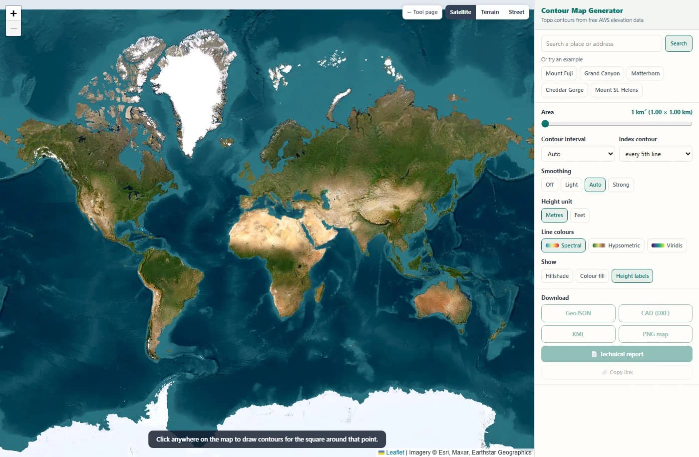
The tool opens on a satellite world map. The panel on the right holds the search box, the example places and all settings. Nothing is drawn until you pick a place.
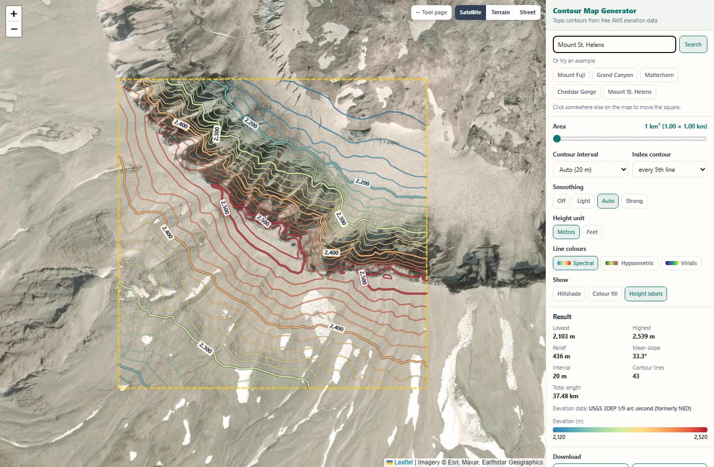
Type a place name and press Enter, or click one of the examples. Here "Mount St. Helens" moves the map to the volcano, and the tool draws contour lines for 1 km² around the result right away.
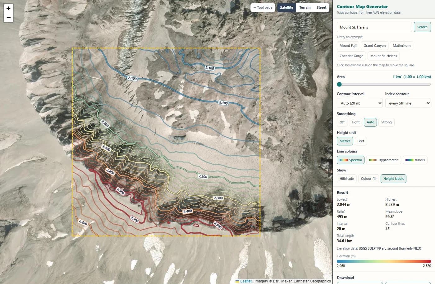
Click anywhere on the map to move the square there. The tool loads the elevation tiles for the new place and draws the lines in a second or two. Index contours are thicker and carry height labels.
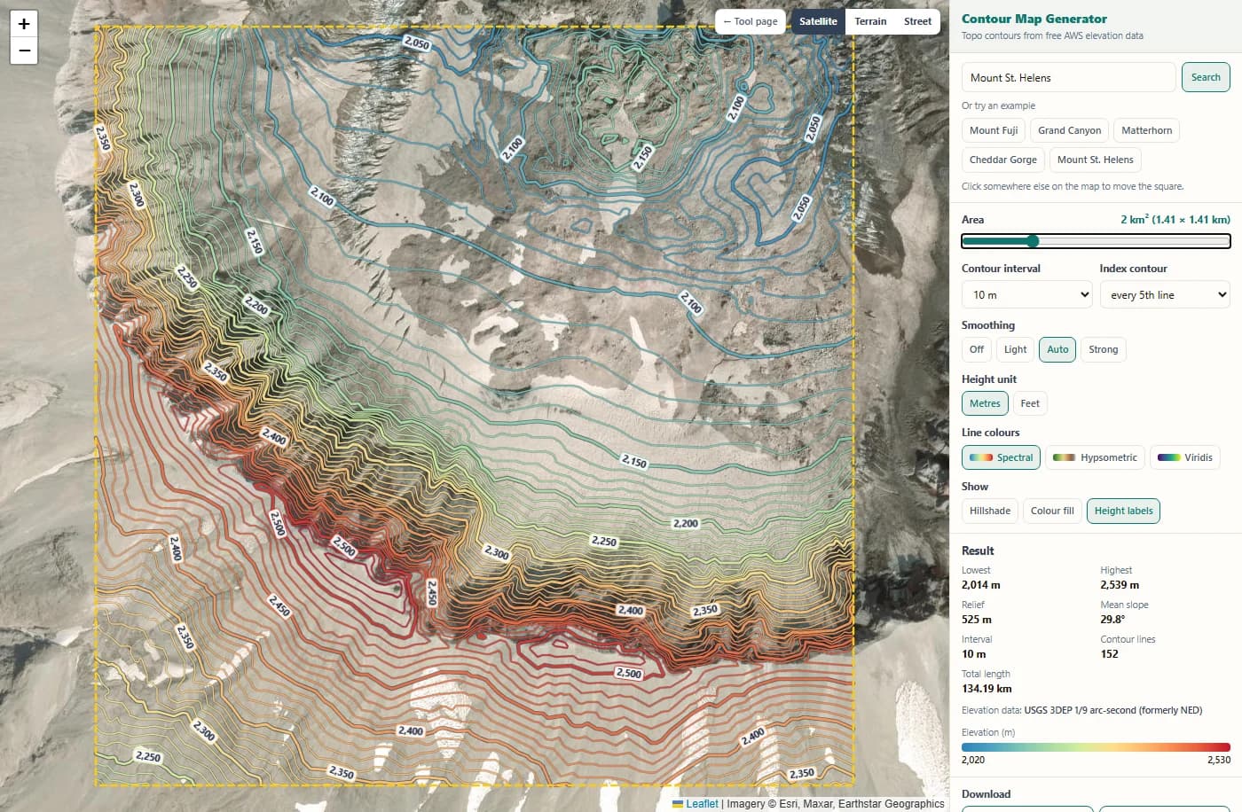
Move the area slider to 2 km² and pick a 10 m interval. The square grows to 1.41 × 1.41 km and the map redraws at once. The result panel shows how many lines you get (here more than 100) and their total length.
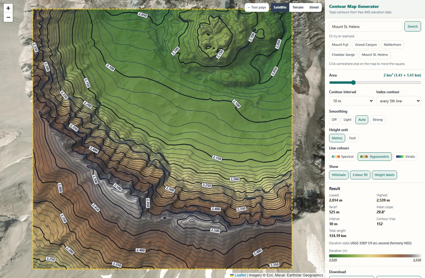
Switch on the hillshade and the colour fill and choose the Hypsometric colours. The fill colours the ground by height, so the lines turn dark for contrast. The legend shows which colour belongs to which height.
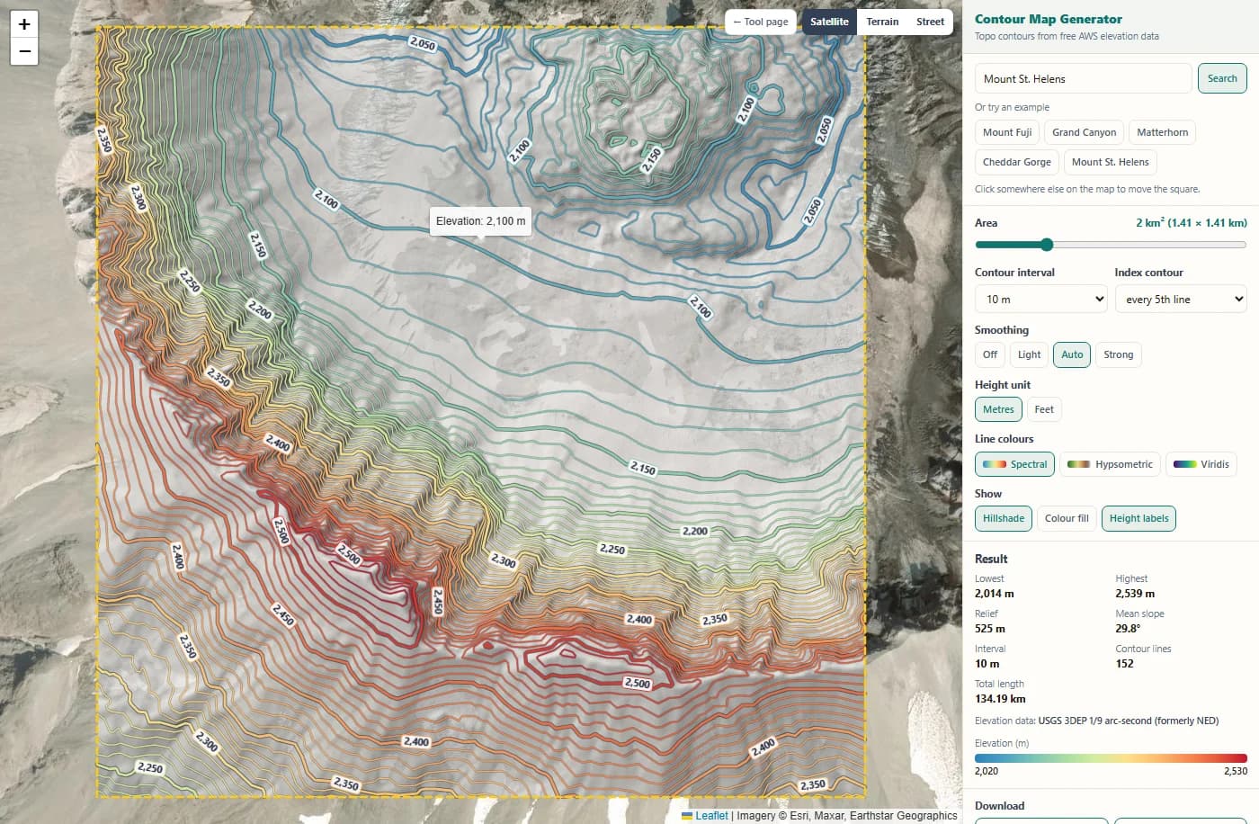
Hover any line to see its exact height. The result panel lists the lowest and highest point, the relief, the mean slope and the elevation datasets used. Here the data is the USGS 3DEP 1/9 arc-second model (about 3 m), which is why the lines show so much detail on the crater wall.
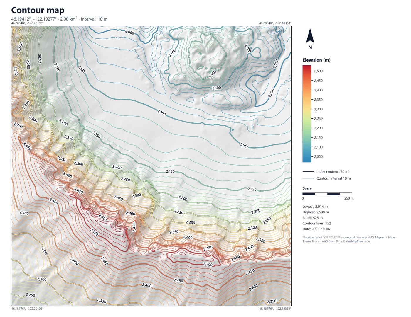
The PNG map is 2200 × 1700 pixels with shaded relief, coloured contours, height labels, a legend, a scale bar, a north arrow and the data credits. It is ready to print or to put in a report.
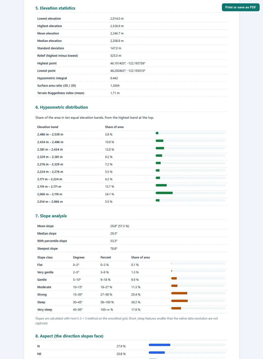
The report gives the elevation, slope, aspect and contour statistics, the processing settings and a plain-language reading of the terrain. Print it or save it as a PDF from the button at the top.
The logic and the math behind the contour lines
A contour line looks simple, but drawing a good one takes several steps. Here is exactly what the tool does with the numbers, from the elevation tile to the finished line.
1. Reading heights from the elevation tiles
The AWS Terrain Tiles store heights inside normal PNG images, in a format called Terrarium. Each pixel has a red, green and blue value from 0 to 255, and the three values together give the height with a precision of 1/256 m (about 4 mm):
height = (R × 256 + G + B / 256) − 32768      (metres)

example pixel  R = 128, G = 100, B = 64
height = (128 × 256 + 100 + 64 / 256) − 32768
       = 32868.25 − 32768
       = 100.25 m
The tool uses zoom level 15, the finest level of the tiles. One tile is 256 × 256 pixels. Each tile also sends a header, x-amz-meta-x-imagery-sources, with the names of the source datasets in it. That is how the report can tell you whether your heights come from a 2 m LIDAR survey or from 30 m SRTM radar data.
2. From your click to a square of grid cells
Your click gives a latitude φ and longitude λ. The square has a side s = √A, where A is the area you chose. The tool turns the half side into degrees with the length of one degree at that latitude, then converts the corners to Web Mercator pixels at zoom 15:
s = √A                         A = 2 km²  →  s = 1414.2 m
Δφ = (s / 2) / (111132.95 − 559.82·cos 2φ + 1.18·cos 4φ)
Δλ = (s / 2) / (111412.84·cos φ − 93.5·cos 3φ)

x = (λ + 180) / 360 × 256 × 2^15
y = (1 − ln(tan φ + sec φ) / π) / 2 × 256 × 2^15

cell size = 40075016.69 × cos φ / (256 × 2^15)
          = 4.78 m at the equator, 3.31 m at 46.2° N (Mount St. Helens)
The grid covers the square plus a margin of 16 cells on every side, so the smoothing and the slope calculation have real neighbours at the edge. Inside 2.3 km the size of a Mercator pixel changes by less than 0.05 %, so every cell can be treated as a square of the same size.
3. Smoothing the height grid
Most elevation data is coarser than the tile pixels. SRTM, for example, has one height every 30 m and whole metres only. Enlarged to 3 m cells, it turns into small flat terraces with 1 m steps, and a contour line drawn on that would zig-zag along every step. A Gaussian filter fixes this. Each cell becomes a weighted average of its neighbours:
G(d) = e^(−d² / 2σ²)                 weight at distance d (cells)
z'(x, y) = Σ G(i)·G(j)·z(x+i, y+j) / Σ G(i)·G(j)     for |i|, |j| ≤ 3σ

auto:  σ = 0.3 × native resolution / cell size   (0.7 to 4 cells)
SRTM 30 m, cell 3.4 m  →  σ = 2.6 cells (9 m)
LIDAR 2 m, cell 3.0 m  →  σ = 0.7 cells (2 m)
The filter is separable, so it runs once along the rows and once along the columns, which is fast. Light halves the automatic σ, Strong doubles it, Off keeps the raw values. Smoothing slightly rounds off sharp summits, so the lowest, highest and mean elevation in the panel and the report are read from the raw data, not the smoothed grid. My take: leave it on Auto unless you have a reason. With LIDAR data it barely touches the lines; with SRTM it is the difference between a usable map and a messy one.
4. Marching squares: finding where a line crosses each cell
For each contour level L, the tool looks at every square of four neighbouring grid points. Each corner is either above or below L, which gives 16 possible cases. Where one corner of an edge is above and the other below, the line crosses that edge, and linear interpolation gives the exact point:
corners  tl  tr        bit = 1 if height ≥ L
         bl  br        case = 8·tl + 4·tr + 2·br + 1·bl   (0 … 15)

crossing on an edge from a to b:
  t = (L − za) / (zb − za)          0 ≤ t ≤ 1
  point = a + t × (b − a)

example  za = 512.0 m, zb = 527.0 m, L = 520 m
  t = (520 − 512) / (527 − 512) = 0.533  → 53 % along the edge
Two cases (5 and 10) are saddles: the two high corners sit opposite each other. A saddle can be joined two ways, so the tool takes the average of the four corners. If the centre is above L, the high corners are connected through the middle; if not, the low corners are. This removes the ambiguity and stops lines from crossing.
5. Joining, clipping and simplifying the lines
Marching squares gives many thousands of tiny segments, one or two per crossed cell. Two neighbouring cells share an edge, so they produce exactly the same crossing point on it. The tool gives every cell edge a number and joins segments that meet on the same edge into one long polyline. When a polyline comes back to its start, it is a closed line around a hilltop or a hollow.
edge id (horizontal) = row × columns + column
edge id (vertical)   = rows × columns + row × columns + column

line clipping (Liang–Barsky):  keep the part with  0 ≤ t ≤ 1  inside the square
simplification (Douglas–Peucker): drop a point if it lies closer
  than 0.2 cells (about 0.6 to 1 m) to the line through its neighbours
Then every line is clipped exactly to the edge of your square, so the CAD and GIS files end on a clean boundary. Finally the Douglas–Peucker method removes points that add no shape, which keeps the files small without changing the drawing. Pieces shorter than 1.5 cells are dropped as noise.
6. Choosing the interval and the index contours
The automatic interval is the smallest round number (1, 2, 2.5, 5, 10, 20, 25, 50, 100 …) that gives at most 25 contour levels over the height range, but not finer than half the typical vertical error of the data. Index contours are the levels that are an exact multiple of the interval times five:
levels  = ⌈zmin / i⌉ × i  …  ⌊zmax / i⌋ × i
index   = level / i  divisible by 5   (or 4, or 10)

example  zmin = 832 m, zmax = 1095 m, relief = 263 m
  i = 5 m  → 53 levels (too many)
  i = 10 m → 26 levels (too many)
  i = 20 m → 13 levels  ✓   index contours at 900 and 1000 m
There is also a rule of thumb from map accuracy standards: the interval should be at least about twice the vertical error of the data. The tool calls this the recommended minimum, shows a warning in the panel when you go finer, and writes it in the report.
7. Slope, aspect and hillshade
Slope, aspect and the hillshade come from the same smoothed grid, using Horn's 3 × 3 method, the one used by most GIS software. For the eight neighbours a to i around a cell (e is the centre):
dz/dx = ((c + 2f + i) − (a + 2d + g)) / (8 × cell)
dz/dy = ((g + 2h + i) − (a + 2b + c)) / (8 × cell)

slope  = atan( √(dz/dx² + dz/dy²) )          degrees
aspect = atan2( −dz/dx, dz/dy )              0° = facing north
slope % = tan(slope) × 100                   45° = 100 %

hillshade = sin(alt)·cos(slope) + cos(alt)·sin(slope)·cos(az − aspect)
            sun azimuth 315° (north-west), altitude 45°
The report sorts every cell into seven slope classes (0 to 2°, 2 to 5°, 5 to 10°, 10 to 15°, 15 to 30°, 30 to 45° and steeper) and eight aspect directions. Cells flatter than 1° have no real direction, so they are counted separately as flat.
8. Terrain numbers in the report
Three more numbers describe the character of the terrain. The hypsometric integral shows whether most of the land is high or low. The surface area ratio compares the real sloping surface with the flat map area. The Terrain Ruggedness Index (Riley, 1999) is the average height difference between a cell and its eight neighbours.
HI  = (mean − min) / (max − min)       0 … 1
      HI > 0.6 plateau-like,  HI < 0.4 valley-like

surface ratio = mean of √(1 + dz/dx² + dz/dy²)
      1.000 flat,  1.155 everywhere 30°

TRI = mean of  Σ |z_neighbour − z_centre| / 8

contour density = total line length / area     (km per km²)
Contour density is a quick roughness check too: flat farmland at a 5 m interval may have 2 to 5 km of contour per km², a steep mountainside 30 km or more.
Download formats in detail
Each download is built in your browser from the same contour lines, so the files always match what you see on the map. Here is what is inside each one and where to use it.
GeoJSON .geojson
Draw contour GeoJSON online and download it as a standard RFC 7946 FeatureCollection. Every contour is a LineString in WGS84 longitude and latitude, with the height as the third coordinate. The properties hold the elevation, the unit, the type (index or intermediate), whether the line is closed, its length in metres and its display colour.
{ "type": "Feature",
  "properties": { "elevation": 1000, "unit": "m", "type": "index",
                  "closed": false, "length_m": 1243.6,
                  "stroke": "#f88d52", "stroke-width": 2.5 },
  "geometry": { "type": "LineString",
                "coordinates": [[-4.0761234, 53.0687456, 1000], …] } }
Use it in QGIS, ArcGIS Pro, Mapbox, Leaflet, deck.gl or geojson.io. The "stroke" property means many web viewers show the lines in the same colours as here.
CAD (DXF) .dxf
The DXF file is written in the AutoCAD R12 ASCII format, which every CAD program can open: AutoCAD, Civil 3D, BricsCAD, DraftSight, LibreCAD, MicroStation, SketchUp (with an importer) and QGIS. Coordinates are in UTM metres for the zone of your square (the EPSG code is in the file name and in a comment at the top of the file), so distances and areas measure correctly in CAD.
Layers   CONTOUR_INDEX          index lines, colour 7
         CONTOUR_INTERMEDIATE   other lines, colour 8
         CONTOUR_LABELS         height text on index lines
         BOUNDARY               the square
Entity   POLYLINE with elevation (group 30) = contour height
         every VERTEX also carries Z = contour height
Because every polyline carries its real elevation, Civil 3D and similar programs can build a surface (TIN) straight from the contours. Each line also gets a colour close to the colour on the map. This is the main reason I built a contour map creator for CAD: most free tools give you a picture or flat lines without heights.
KML .kml
The KML file opens in Google Earth, Google My Maps, ArcGIS Earth and most GIS programs. The lines sit in two folders, index and intermediate contours, plus the square as a boundary. Each line is named by its height and keeps its colour and line width. Heights are written in metres, as KML requires, and the lines are clamped to the ground so they drape over the 3D terrain in Google Earth.
In Google Earth Pro, tilt the view after opening the file: the contours lie on the 3D ground, which makes it easy to check them against the real landscape.
PNG map .png
The contour map creator PNG export is a 2200 × 1700 pixel image, sharp enough to print on A4 or Letter paper at 200 dpi. It has a title, the centre coordinates, a soft hillshade, the coloured contours with labelled index lines, the coordinates of the corners, a vertical colour legend, a line key, a scale bar, a north arrow, the key numbers and the data credits.
Put it straight into a report, a presentation or a planning application. The background is drawn from the height grid itself, so the image has no copyright limits from a third-party base map.
Technical report .html
The report is one HTML file that opens in any browser and prints neatly to PDF. It has twelve sections: project summary, the map, the elevation datasets, processing settings, elevation statistics, the hypsometric distribution, slope classes, aspect, contour statistics with the length of every level, a plain-language interpretation, accuracy notes and the data credits.
The text adapts to the result. A flat site gets a note about drainage, a steep one tells you how much of the land is steeper than 15°, and if you chose an interval finer than the data supports, the report says so.
Need the lines in Shapefile format? Open the GeoJSON in QGIS and use Export → Save Features As → ESRI Shapefile. To check a file quickly, drop it into the GeoJSON Viewer or the DXF Viewer on this site. File names include the centre point and the interval, so several downloads never overwrite each other.
Who uses contour maps, and for what
Contour lines are the common language of anyone who works with the shape of the ground. Here are the jobs this contour map generator is used for most.
- Architects and landscape designers. Get the contours of a building plot into AutoCAD before the first sketch, to place the house, plan terraces and check views. The DXF opens at the right size and position.
- Civil engineers and early feasibility. Check the slope of a road, pipeline or drainage route before paying for a survey, estimate cut and fill, and build a rough TIN surface in Civil 3D from the contours.
- Solar and wind projects. Slope and aspect decide where panels and turbines can go. The report gives the share of land below 5° and the main slope direction in one page.
- Hikers, runners and trail builders. Make a topo map of a route or a summit area, print the PNG, or load the GeoJSON into a GPS app. Closed lines show hilltops and hollows at a glance.
- Farmers and soil and water work. Plan contour ploughing, swales, ponds and terraces. A 1 m or 2 m interval on good data shows where water will run.
- Drone pilots and surveyors. Plan flight heights over hilly ground, or compare a fresh drone model with the public elevation data for the same square.
- Teachers and students. Show how contour lines relate to the shape of a valley or a volcano with the hillshade switched on and off, and use the report for geography and GIS assignments.
- Real estate and land buyers. See in a minute whether a plot is flat, gently sloping or steep, and add a clean contour map to a listing or a land report.
- Game and 3D artists. Use real terrain shapes as a base for game levels, model railways and 3D prints: the KML and GeoJSON carry the heights.
Frequently asked questions about contours and this tool
The 20 questions people ask most about contour maps, topo maps and this contour generator.
1. What is a contour line?
A contour line joins points of the same height above sea level. If you walked along one, you would never go up or down. The lines on a map are a stack of these slices through the ground, usually at a fixed height step called the contour interval.
2. What is the contour interval, and which one should I choose?
The interval is the height difference between two neighbouring lines. Small intervals (1 to 2 m) show detail on gentle ground; large ones (20 to 50 m) keep steep mountains readable. Start with Auto: it gives at most 25 levels and respects the quality of the data. For CAD work on a building plot, 1 m is common, but only if the report says your data is fine enough.
3. What are index contours?
Index contours are every fifth line (here you can also choose every fourth or tenth). They are drawn thicker and carry the height label, so you can count lines quickly from a known height. On a 10 m interval map, the index contours are at 50 m steps: 500, 550, 600 and so on.
4. How do I read slope from contour lines?
Close lines mean steep ground, wide gaps mean flat ground. You can measure it too: slope = interval ÷ horizontal distance between two lines. With a 10 m interval and lines 50 m apart, the slope is 10 ÷ 50 = 20 % or about 11.3°. The report gives the slope statistics for the whole square.
5. How do I tell a hill from a hollow?
Both appear as closed rings. If the heights increase towards the centre, it is a hill; if they decrease, it is a hollow or a depression. Turn on the height labels and the colour fill, or hover the lines: the colour scale makes it obvious.
6. What do V-shaped and U-shaped contours mean?
Where contours form a V, the V points uphill along a stream valley; water flows out of the open end. A U or rounded shape pointing downhill is a ridge or spur. This is the quickest way to find drainage lines on any topo map.
7. What is the difference between a contour map and a topo map?
A topographic (topo) map shows the land surface in general, usually with contour lines plus roads, rivers, buildings and names. A contour map shows only the height lines. This tool makes a contour map, and the satellite or terrain base map adds the topo context on screen.
8. Where does the elevation data come from?
From the AWS Terrain Tiles, a free open dataset made by Mapzen (Tilezen project) and hosted on the AWS Open Data Registry. It merges the best public elevation data for each place: USGS 3DEP in the USA, Environment Agency LIDAR in England, EU-DEM in Europe, SRTM for most of the world, and several national models. The report lists the datasets used for your square.
9. How accurate are the contour lines?
It depends on the source. LIDAR (England, parts of the USA) is accurate to about 15 to 50 cm; national 5 to 10 m models to 1 to 2 m; SRTM radar data typically to 5 to 10 m, worse in forests, towns and very steep ground. The lines are good for planning, studies and maps, not for construction setting-out. The report names the source and a recommended minimum interval.
10. Why do the contours look smooth when the data is 30 m?
The tool smooths the height grid with a Gaussian filter before it draws the lines. Without it, coarse data enlarged to 3 to 5 m cells creates staircase lines. Smoothing does not add accuracy; it removes artefacts. You can switch it to Light or Off to see the raw result.
11. Can I open the contours in AutoCAD or Civil 3D?
Yes. Download the CAD (DXF) file and open it directly. The lines are on separate layers for index and intermediate contours, in UTM metres, and every polyline has its elevation set, so Civil 3D can create a surface from them. The UTM zone (EPSG code) is in the file name.
12. Why are the DXF coordinates in UTM and not latitude and longitude?
CAD programs measure in flat units such as metres. Latitude and longitude are angles, so distances and areas would come out wrong. UTM is a metric grid used worldwide, accurate to a fraction of a millimetre per metre across a 2 km square. If you need a national grid, re-project the GeoJSON in QGIS.
13. How do I draw contour GeoJSON online and use it in QGIS?
Click the map, adjust the interval, and press GeoJSON. In QGIS, drag the file onto the map. To label it, use the "elevation" field; to style it, use "type" (index or intermediate) or "elevation" with a graduated colour ramp. The file is plain WGS84, so it lines up with any base map.
14. Can I get contours in feet?
Yes. Set the height unit to Feet. The intervals change to feet values (1, 2, 5, 10, 20 ft and up), labels and statistics are in feet, and the DXF elevations are in feet. The DXF X and Y coordinates stay in UTM metres. KML heights are always in metres, because KML requires it.
15. Why is the area limited to 5 km²?
A 5 km² square already needs 4 to 9 elevation tiles and about a quarter of a million height cells at full resolution, all processed in your browser. Larger areas would be slow on phones and would give crowded maps. For a bigger site, make several squares side by side; the edges are clipped exactly, so they join cleanly.
16. Can I make contours below sea level?
Yes. Over the sea the tiles contain bathymetry from ETOPO1 and other sources, so you get depth contours with negative heights. Their resolution is much coarser (about 1.8 km for ETOPO1), so treat sea contours as a rough picture only.
17. Is the contour map generator really free? Do I need an account?
It is free, with no account, no watermark on the PNG and no limit on downloads. The elevation tiles are open data on AWS, and all processing runs in your browser, so there is no server cost to pass on to you.
18. Can I use the downloaded maps in commercial work?
Yes. The elevation data is open and may be used commercially, but you must credit the sources. The report and the PNG already contain the required credits; keep them, or copy the credit lines from the "Data sources" section below into your own document.
19. Why do some areas show blocky or striped lines?
Where two datasets meet (for example at a border or a coastline), or where SRTM has filled gaps in mountains and deserts, the data itself can have steps or flat patches. Try the Strong smoothing, or a larger interval, and check the datasets listed in the result panel.
20. How do I print a contour map at a set scale?
The PNG map is 1500 pixels across for the square. For a 1 × 1 km square printed 15 cm wide, the scale is 1:6,667; for 2.24 km it is about 1:15,000. Use the scale bar on the map to check after printing, and print at 100 % size without "fit to page".
Data sources and credits
The heights come from the AWS Terrain Tiles. The tiles combine many public elevation datasets, and their licences ask for the credits below. The datasets actually used for your square are named in the result panel, the PNG and the report.
- Terrain Tiles on AWS (Mapzen / Tilezen Joerd) · AWS Open Data, terms of each sourceTerrain Tiles: the merged, global elevation tiles in Terrarium PNG format that this tool reads, built by Mapzen's Joerd project (Tilezen) and hosted free on the AWS Open Data Registry.
- USGS 3DEP (formerly NED) · Public domain (U.S. Government)United States: 3DEP (formerly NED) at 1/3 arc-second (about 10 m) and 1/9 arc-second (about 3 m), courtesy of the U.S. Geological Survey.
- SRTM (NASA / USGS) · Public domain (U.S. Government)Most of the world between 60° N and 56° S: SRTM 1 arc-second (about 30 m) radar data, courtesy of the U.S. Geological Survey.
- GMTED2010 (USGS) · Public domain (U.S. Government)Global low zooms: GMTED2010, courtesy of the U.S. Geological Survey.
- ETOPO1 (NOAA NCEI) · Public domain (U.S. Government)Oceans: ETOPO1 global relief (about 1.8 km), U.S. National Oceanic and Atmospheric Administration.
- EU-DEM (Copernicus) · Copernicus free and open data policyEurope: EU-DEM, produced using Copernicus data and information funded by the European Union.
- Environment Agency LIDAR (England) · Open Government LicenceEngland: Environment Agency LIDAR DTM at 2 m, © Environment Agency copyright and/or database right 2015. All rights reserved.
- ArcticDEM (Polar Geospatial Center) · Free use with acknowledgementArctic (north of 60°): ArcticDEM 5 m mosaics, created from DigitalGlobe, Inc. imagery and funded under NSF awards 1043681, 1559691 and 1542736.
- Canadian Digital Elevation Model (NRCan) · Open Government Licence – CanadaCanada: Canadian Digital Elevation Model, contains information licensed under the Open Government Licence – Canada.
- Geoscience Australia · CC BY 4.0Australia: © Commonwealth of Australia (Geoscience Australia) 2017.
- DGM Österreich (data.gv.at) · CC BY 4.0Austria: © offene Daten Österreichs – Digitales Geländemodell (DGM) Österreich.
- INEGI Continental Relief (Mexico) · INEGI terms of free useMexico: INEGI, Continental relief, 2016.
- Land Information New Zealand (LINZ) · Crown copyrightNew Zealand: Copyright 2011 Crown copyright (c) Land Information New Zealand and the New Zealand Government. All rights reserved.
- Kartverket (Norway) · CC BY 4.0Norway: © Kartverket.
If you publish a map made with this tool, keep the credit line that comes with the PNG and the report. It already lists the datasets used for your area.
Software and map credits
The tool is built on open software and services:
- Leaflet 1.9 · BSD-2-ClauseInteractive map, polylines, the square and the image overlays.
- proj4js · MITConverts the CAD export to UTM metres for the zone of your square.
- Esri World Imagery and World Hillshade · Esri terms of useSatellite base map (World Imagery) and the Terrain base map (World Hillshade).
- Protomaps (hosted by KONAKTIVE), CARTO, OpenStreetMap · ODbL and provider termsStreet base map: own vector tiles hosted by KONAKTIVE, with CARTO and OpenStreetMap as fallback.
- Place search through this site's own address service.
The contour engine (decoding, smoothing, marching squares, clipping, statistics and all exports) was written for this site and runs entirely in your browser.
Related elevation and map tools
Contours are made from public elevation models and are approximate. Do not use them for construction, navigation or legal boundaries without a professional survey. Elevation data: Terrain Tiles (Mapzen / Tilezen) on AWS. Map tiles © OpenStreetMap contributors, drawn with Protomaps (hosted by KONAKTIVE), with CARTO as the fallback. Satellite imagery: Esri.